Importance of Velocity of Propagation in TDR Method for UG cable fault location

In the previous blog, we concluded our three-part series on underground cable fault location. To review, we discussed the types of cable faults, methodology for locating cable faults, fault finding through Pre-location techniques and cable route tracing, pinpointing, cable identification and repair and re-test.

In Part-2 of our 3 part series, we introduced the methodology of Pre-location using Time Domain Reflectometer (TDR) method. In this blog post, we will share our knowledge on accurately setting velocity of propagation in TDR method and the importance for the same.

Velocity of Propagation in TDR Method

For accurate fault location for underground cables using TDR method, it is essential that the correct velocity be applied.

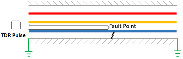
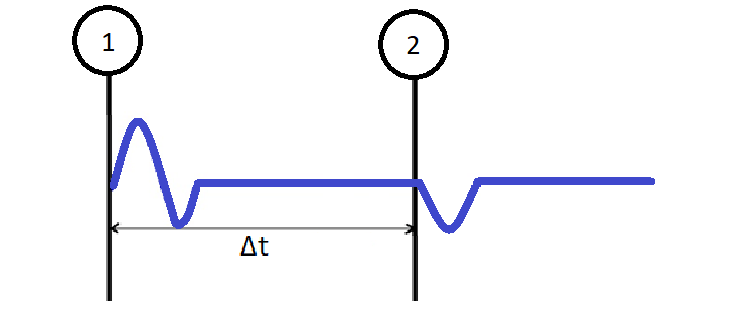
To review the TDR method, a low voltage, high frequency pulse is sent into the cable from one end. If any impedance mismatch occurs in the cable, then part or all of the pulse energy is reflected back towards the TDR (Prelocator) unit. The time taken by pulse having particular velocity of propagation for returning back to source end is the measure of the fault distance. The velocity of propagation is constant for a particular cable and depends on the cable dielectric/insulation material, insulation thickness, conductor size, conductor resistance manufacturing process, etc.

The velocity of propagation (V) of TDR pulse in a cable is the ratio of velocity of light in free space (C) and square root of relative permittivity (εr) of the dielectric / insulation of cable. The actual fault distance is calculated by multiplying travelling time of pulse in microseconds and velocity of propagation in meters per microsecond.

As the pulse travels to fault point and returns back, the value of velocity of propagation is used as half of the actual i.e., V/2 in most of the instruments, for ease in calculations. While some of the manufacturers use actual value of velocity of propagation(V) as input and display the distance value which is half of the calculated value.

Velocity Factor (VF)

Velocity of propagation is also expressed in terms of velocity of light in free space. The ratio of the propagation velocity of electromagnetic wave (TDR Pulse) in the cable (V) and the velocity of light in free space (C≈300m/μs) is called as Velocity Factor (VF). It is calculated in m/μs. The unknown value of VF for cable under test can be determined by TDR testing of a known length of that cable and adjust the VF until the distance displayed to the end of the cable is correct.

Propagation Factor (PF)

The propagation factor is the velocity of light in free space in m/μs (C) divided by the velocity of propagation of TDR pulse in a given cable in m/μs (V). Propagation factor is also called “shortening factor”.

Percentage Velocity (VoP%)

The percentage of the velocity of propagation of TDR pulse (m/μs) in a given cable with respect to velocity of light in free space is called VoP (%). It is simply calculated by multiplying velocity factor by 100.

Example

To better illuminate our discussion, consider that a particular type of cable is having the Velocity of Propagation as 172m/μs, by considering the speed of light in free space as 300m/μs, the various relations of VOP will be as below:

• Velocity of Propagation, V = 172m/μs
• Velocity Factor, VF = V/C =172 / 300 = 0.573
• Propagation Factor, PF = C/V=300 / 172=1.744
• VoP (%) = VF x 100 = 0.573 * 100 = 57.3

The table below illustrates the typical values based on types of cable insulation and dielectric/insulation type:

Cable Type	Dielectric/ insulation Type	Velocity Factor	Propagation Factor	VoP(%)	V (m/μs)	V/2 (m/μs)
Power	Impregnated Paper / PIC	0.5 to 0.57	2 to 1.75	50 to 57	150 to 171	75 to 85.5
Power	PVC	0.51 to .58	1.97 to 1.715	51 to 58	152 to 175	76 to 87.5
Power	Paper Oil Filled	0.72 to 0.84	1.38 to 1.19	72 to 84	216 to 252	108 to 126
Power	PE	0.46 to 0.58	1.72 to 2.15	46 to 58	139.2 to 174	69.6 to 87
Power	XLPE	0.54 to 0.62	1.92 to 1.61	54 to 62	156 to 186	78 to 93
Power	EPR	0.45 to 0.57	2.22 to 1.75	45 to 57	135 to 171	67.5 to 85.5
Twisted Pair	Polyethylene	0.64 to 0.67	1.56 to 1.49	64 to 67	192 to 201	96 to 100.5
Twisted Pair	PTFE	≈0.71	≈1.41	≈71	≈213	≈106.5
Twisted Pair	Dry Paper	0.72 to 0.88	1.38 to 1.14	72 to 88	216 to 264	108 to 132
Telecom	PIC	0.65 to 0.72	1.54 to 1.39	65 to 72	195 to 216	97.5 to 108
Telecom	Pulp	0.66 to 0.71	1.51 to 1.41	66 to 71	198 to 213	99 to 106.5
Telecom	Gel Filled	0.58 to 0.68	1.72 to 1.47	58 to 68	174 to 204	87 to 102
Telecom	Co-Axial	0.82 to 0.98	1.22 to 1.02	82 to 98	246 to 294	123 to 147

Summary

By correctly applying the velocity of propagation in TDR method as discussed above, we can ensure the accuracy of underground cable fault location using TDR method.

For more information on SCOPE cable fault locator capabilities, please visit https://www.scopetnm.com/test-and-measurements or check our recent webinar on cable fault location on SCOPE’s YouTube channel. We also invite you to e-mail us at marketing@scopetnm.com for any queries, product quotations or services.